Bayesian Poisson Regression
This notebook is ported from the example notebook of PyMC3 on Poisson Regression.
Poisson Regression is a technique commonly used to model count data. Some of the applications include predicting the number of people defaulting on their loans or the number of cars running on a highway on a given day. This example describes a method to implement the Bayesian version of this technique using Turing.
We will generate the dataset that we will be working on which describes the relationship between number of times a person sneezes during the day with his alcohol consumption and medicinal intake.
We start by importing the required libraries.
#Import Turing, Distributions and DataFrames
using Turing, Distributions, DataFrames, Distributed

# Import MCMCChain, Plots, and StatsPlots for visualizations and diagnostics.
using MCMCChains, Plots, StatsPlots

# Set a seed for reproducibility.
using Random
Random.seed!(12);
Generating data
We start off by creating a toy dataset. We take the case of a person who takes medicine to prevent excessive sneezing. Alcohol consumption increases the rate of sneezing for that person. Thus, the two factors affecting the number of sneezes in a given day are alcohol consumption and whether the person has taken his medicine. Both these variable are taken as boolean valued while the number of sneezes will be a count valued variable. We also take into consideration that the interaction between the two boolean variables will affect the number of sneezes
5 random rows are printed from the generated data to get a gist of the data generated.
theta_noalcohol_meds = 1    # no alcohol, took medicine
theta_alcohol_meds = 3      # alcohol, took medicine
theta_noalcohol_nomeds = 6  # no alcohol, no medicine
theta_alcohol_nomeds = 36   # alcohol, no medicine

# no of samples for each of the above cases
q = 100

#Generate data from different Poisson distributions
noalcohol_meds = Poisson(theta_noalcohol_meds)
alcohol_meds = Poisson(theta_alcohol_meds)
noalcohol_nomeds = Poisson(theta_noalcohol_nomeds)
alcohol_nomeds = Poisson(theta_alcohol_nomeds)

nsneeze_data = vcat(
    rand(noalcohol_meds, q),
    rand(alcohol_meds, q),
    rand(noalcohol_nomeds, q),
    rand(alcohol_nomeds, q),
)
alcohol_data = vcat(zeros(q), ones(q), zeros(q), ones(q))
meds_data = vcat(zeros(q), zeros(q), ones(q), ones(q))

df = DataFrame(;
    nsneeze=nsneeze_data,
    alcohol_taken=alcohol_data,
    nomeds_taken=meds_data,
    product_alcohol_meds=meds_data .* alcohol_data,
)
df[sample(1:nrow(df), 5; replace=false), :]
5×4 DataFrame
 Row │ nsneeze  alcohol_taken  nomeds_taken  product_alcohol_meds
     │ Int64    Float64        Float64       Float64
─────┼────────────────────────────────────────────────────────────
   1 │      22            1.0           1.0                   1.0
   2 │       3            1.0           0.0                   0.0
   3 │       3            1.0           0.0                   0.0
   4 │       4            1.0           0.0                   0.0
   5 │       2            0.0           0.0                   0.0
Visualisation of the dataset
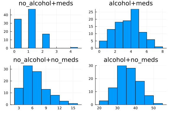
We plot the distribution of the number of sneezes for the 4 different cases taken above. As expected, the person sneezes the most when he has taken alcohol and not taken his medicine. He sneezes the least when he doesn't consume alcohol and takes his medicine.
#Data Plotting

p1 = Plots.histogram(
    df[(df[:, :alcohol_taken] .== 0) .& (df[:, :nomeds_taken] .== 0), 1];
    title="no_alcohol+meds",
)
p2 = Plots.histogram(
    (df[(df[:, :alcohol_taken] .== 1) .& (df[:, :nomeds_taken] .== 0), 1]);
    title="alcohol+meds",
)
p3 = Plots.histogram(
    (df[(df[:, :alcohol_taken] .== 0) .& (df[:, :nomeds_taken] .== 1), 1]);
    title="no_alcohol+no_meds",
)
p4 = Plots.histogram(
    (df[(df[:, :alcohol_taken] .== 1) .& (df[:, :nomeds_taken] .== 1), 1]);
    title="alcohol+no_meds",
)
plot(p1, p2, p3, p4; layout=(2, 2), legend=false)
We must convert our DataFrame data into the Matrix form as the manipulations that we are about are designed to work with Matrix data. We also separate the features from the labels which will be later used by the Turing sampler to generate samples from the posterior.
# Convert the DataFrame object to matrices.
data = Matrix(df[:, [:alcohol_taken, :nomeds_taken, :product_alcohol_meds]])
data_labels = df[:, :nsneeze]
data
400×3 Matrix{Float64}:
 0.0  0.0  0.0
 0.0  0.0  0.0
 0.0  0.0  0.0
 0.0  0.0  0.0
 0.0  0.0  0.0
 0.0  0.0  0.0
 0.0  0.0  0.0
 0.0  0.0  0.0
 0.0  0.0  0.0
 0.0  0.0  0.0
 ⋮
 1.0  1.0  1.0
 1.0  1.0  1.0
 1.0  1.0  1.0
 1.0  1.0  1.0
 1.0  1.0  1.0
 1.0  1.0  1.0
 1.0  1.0  1.0
 1.0  1.0  1.0
 1.0  1.0  1.0
We must recenter our data about 0 to help the Turing sampler in initialising the parameter estimates. So, normalising the data in each column by subtracting the mean and dividing by the standard deviation:
# # Rescale our matrices.
data = (data .- mean(data; dims=1)) ./ std(data; dims=1)
400×3 Matrix{Float64}:
 -0.998749  -0.998749  -0.576628
 -0.998749  -0.998749  -0.576628
 -0.998749  -0.998749  -0.576628
 -0.998749  -0.998749  -0.576628
 -0.998749  -0.998749  -0.576628
 -0.998749  -0.998749  -0.576628
 -0.998749  -0.998749  -0.576628
 -0.998749  -0.998749  -0.576628
 -0.998749  -0.998749  -0.576628
 -0.998749  -0.998749  -0.576628
  ⋮
  0.998749   0.998749   1.72988
  0.998749   0.998749   1.72988
  0.998749   0.998749   1.72988
  0.998749   0.998749   1.72988
  0.998749   0.998749   1.72988
  0.998749   0.998749   1.72988
  0.998749   0.998749   1.72988
  0.998749   0.998749   1.72988
  0.998749   0.998749   1.72988
Declaring the Model: Poisson Regression
Our model, poisson_regression takes four arguments:
xis our set of independent variables;yis the element we want to predict;nis the number of observations we have; andσ²is the standard deviation we want to assume for our priors.
Within the model, we create four coefficients (b0, b1, b2, and b3) and assign a prior of normally distributed with means of zero and standard deviations of σ². We want to find values of these four coefficients to predict any given y.
Intuitively, we can think of the coefficients as:
b1is the coefficient which represents the effect of taking alcohol on the number of sneezes;b2is the coefficient which represents the effect of taking in no medicines on the number of sneezes;b3is the coefficient which represents the effect of interaction between taking alcohol and no medicine on the number of sneezes;
The for block creates a variable theta which is the weighted combination of the input features. We have defined the priors on these weights above. We then observe the likelihood of calculating theta given the actual label, y[i].
# Bayesian poisson regression (LR)
@model function poisson_regression(x, y, n, σ²)
    b0 ~ Normal(0, σ²)
    b1 ~ Normal(0, σ²)
    b2 ~ Normal(0, σ²)
    b3 ~ Normal(0, σ²)
    for i in 1:n
        theta = b0 + b1 * x[i, 1] + b2 * x[i, 2] + b3 * x[i, 3]
        y[i] ~ Poisson(exp(theta))
    end
end;
Sampling from the posterior
We use the NUTS sampler to sample values from the posterior. We run multiple chains using the MCMCThreads() function to nullify the effect of a problematic chain. We then use the Gelman, Rubin, and Brooks Diagnostic to check the convergence of these multiple chains.
# Retrieve the number of observations.
n, _ = size(data)

# Sample using NUTS.

num_chains = 4
m = poisson_regression(data, data_labels, n, 10)
chain = sample(m, NUTS(), MCMCThreads(), 2_500, num_chains; discard_adapt=false)
Chains MCMC chain (2500×16×4 Array{Float64, 3}):

Iterations        = 1:1:2500
Number of chains  = 4
Samples per chain = 2500
Wall duration     = 11.3 seconds
Compute duration  = 10.76 seconds
parameters        = b0, b1, b2, b3
internals         = lp, n_steps, is_accept, acceptance_rate, log_density, h
amiltonian_energy, hamiltonian_energy_error, max_hamiltonian_energy_error,
tree_depth, numerical_error, step_size, nom_step_size

Summary Statistics
  parameters      mean       std      mcse    ess_bulk   ess_tail      rhat
    ⋯
      Symbol   Float64   Float64   Float64     Float64    Float64   Float64
    ⋯

          b0    1.4892    0.7982    0.0576   1008.1853   307.0725    1.0033
    ⋯
          b1    0.5061    1.2211    0.0899   1072.4721   331.4062    1.0036
    ⋯
          b2    0.9299    0.8520    0.0560    819.5763   339.1922    1.0039
    ⋯
          b3    0.3477    1.3250    0.0986   1171.5035   346.7815    1.0036
    ⋯
                                                                1 column om
itted

Quantiles
  parameters      2.5%     25.0%     50.0%     75.0%     97.5%
      Symbol   Float64   Float64   Float64   Float64   Float64

          b0    1.4899    1.5669    1.5896    1.6116    1.6538
          b1    0.4865    0.6080    0.6491    0.6911    0.7772
          b2    0.8555    0.9526    0.9907    1.0327    1.1134
          b3    0.0790    0.1608    0.1993    0.2376    0.3468
Viewing the Diagnostics
We use the Gelman, Rubin, and Brooks Diagnostic to check whether our chains have converged. Note that we require multiple chains to use this diagnostic which analyses the difference between these multiple chains.
We expect the chains to have converged. This is because we have taken sufficient number of iterations (1500) for the NUTS sampler. However, in case the test fails, then we will have to take a larger number of iterations, resulting in longer computation time.
gelmandiag(chain)
Gelman, Rubin, and Brooks diagnostic
  parameters      psrf    psrfci
      Symbol   Float64   Float64

          b0    1.0707    1.0762
          b1    1.1196    1.1391
          b2    1.0974    1.1293
          b3    1.1113    1.1349
From the above diagnostic, we can conclude that the chains have converged because the PSRF values of the coefficients are close to 1.
So, we have obtained the posterior distributions of the parameters. We transform the coefficients and recover theta values by taking the exponent of the meaned values of the coefficients b0, b1, b2 and b3. We take the exponent of the means to get a better comparison of the relative values of the coefficients. We then compare this with the intuitive meaning that was described earlier.
# Taking the first chain
c1 = chain[:, :, 1]

# Calculating the exponentiated means
b0_exp = exp(mean(c1[:b0]))
b1_exp = exp(mean(c1[:b1]))
b2_exp = exp(mean(c1[:b2]))
b3_exp = exp(mean(c1[:b3]))

print("The exponent of the meaned values of the weights (or coefficients are): \n")
println("b0: ", b0_exp)
println("b1: ", b1_exp)
println("b2: ", b2_exp)
println("b3: ", b3_exp)
print("The posterior distributions obtained after sampling can be visualised as :\n")
The exponent of the meaned values of the weights (or coefficients are):
b0: 4.303252312705445
b1: 1.5007195233632782
b2: 2.424891112849863
b3: 1.576824642128675
The posterior distributions obtained after sampling can be visualised as :
Visualising the posterior by plotting it:
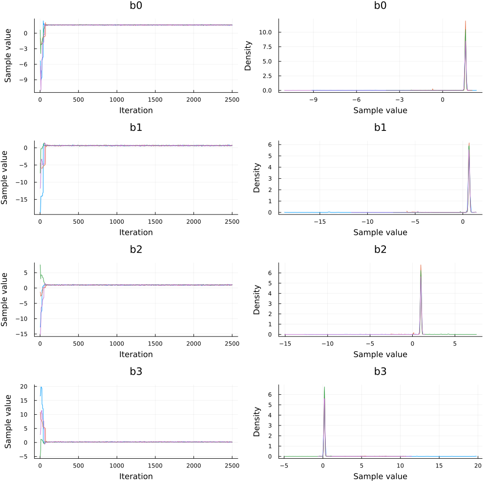
plot(chain)
Interpreting the Obtained Mean Values
The exponentiated mean of the coefficient b1 is roughly half of that of b2. This makes sense because in the data that we generated, the number of sneezes was more sensitive to the medicinal intake as compared to the alcohol consumption. We also get a weaker dependence on the interaction between the alcohol consumption and the medicinal intake as can be seen from the value of b3.
Removing the Warmup Samples
As can be seen from the plots above, the parameters converge to their final distributions after a few iterations. The initial values during the warmup phase increase the standard deviations of the parameters and are not required after we get the desired distributions. Thus, we remove these warmup values and once again view the diagnostics. To remove these warmup values, we take all values except the first 200. This is because we set the second parameter of the NUTS sampler (which is the number of adaptations) to be equal to 200.
chains_new = chain[201:end, :, :]
Chains MCMC chain (2300×16×4 Array{Float64, 3}):

Iterations        = 201:1:2500
Number of chains  = 4
Samples per chain = 2300
Wall duration     = 11.3 seconds
Compute duration  = 10.76 seconds
parameters        = b0, b1, b2, b3
internals         = lp, n_steps, is_accept, acceptance_rate, log_density, h
amiltonian_energy, hamiltonian_energy_error, max_hamiltonian_energy_error,
tree_depth, numerical_error, step_size, nom_step_size

Summary Statistics
  parameters      mean       std      mcse    ess_bulk    ess_tail      rha
t   ⋯
      Symbol   Float64   Float64   Float64     Float64     Float64   Float6
4   ⋯

          b0    1.5904    0.0318    0.0006   3018.5987   3558.1775    1.001
6   ⋯
          b1    0.6517    0.0600    0.0013   2126.5897   3007.0412    1.002
9   ⋯
          b2    0.9929    0.0568    0.0012   2123.3159   3344.1968    1.003
1   ⋯
          b3    0.1974    0.0555    0.0012   2077.3817   3057.5515    1.003
0   ⋯
                                                                1 column om
itted

Quantiles
  parameters      2.5%     25.0%     50.0%     75.0%     97.5%
      Symbol   Float64   Float64   Float64   Float64   Float64

          b0    1.5272    1.5691    1.5907    1.6120    1.6521
          b1    0.5393    0.6111    0.6501    0.6911    0.7731
          b2    0.8846    0.9548    0.9912    1.0316    1.1050
          b3    0.0837    0.1611    0.1985    0.2357    0.3013
plot(chains_new)
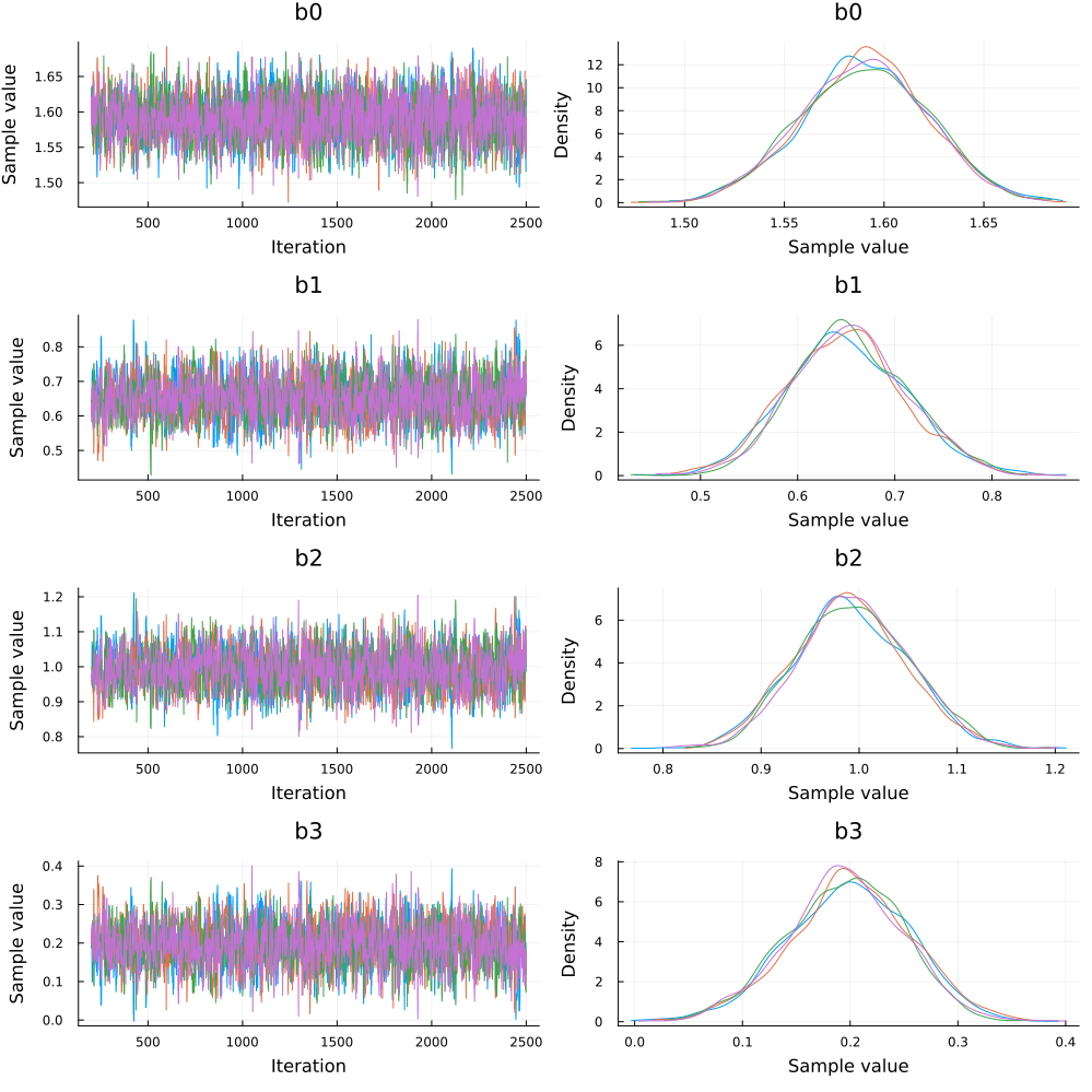
As can be seen from the numeric values and the plots above, the standard deviation values have decreased and all the plotted values are from the estimated posteriors. The exponentiated mean values, with the warmup samples removed, have not changed by much and they are still in accordance with their intuitive meanings as described earlier.
Appendix
These tutorials are a part of the TuringTutorials repository, found at: https://github.com/TuringLang/TuringTutorials.
To locally run this tutorial, do the following commands:
using TuringTutorials
TuringTutorials.weave("07-poisson-regression", "07_poisson-regression.jmd")
Computer Information:
Julia Version 1.9.3
Commit bed2cd540a1 (2023-08-24 14:43 UTC)
Build Info:
  Official https://julialang.org/ release
Platform Info:
  OS: Linux (x86_64-linux-gnu)
  CPU: 128 × AMD EPYC 7502 32-Core Processor
  WORD_SIZE: 64
  LIBM: libopenlibm
  LLVM: libLLVM-14.0.6 (ORCJIT, znver2)
  Threads: 1 on 16 virtual cores
Environment:
  JULIA_CPU_THREADS = 16
  JULIA_DEPOT_PATH = /cache/julia-buildkite-plugin/depots/7aa0085e-79a4-45f3-a5bd-9743c91cf3da
  JULIA_IMAGE_THREADS = 1
Package Information:
Status `/cache/build/default-amdci4-1/julialang/turingtutorials/tutorials/07-poisson-regression/Project.toml`
  [a93c6f00] DataFrames v1.6.1
  [b4f34e82] Distances v0.10.10
  [31c24e10] Distributions v0.25.102
  [38e38edf] GLM v1.9.0
  [c7f686f2] MCMCChains v6.0.3
  [cc2ba9b6] MLDataUtils v0.5.4
  [872c559c] NNlib v0.9.7
  [91a5bcdd] Plots v1.39.0
  [ce6b1742] RDatasets v0.7.7
  [4c63d2b9] StatsFuns v1.3.0
  [f3b207a7] StatsPlots v0.15.6
  [fce5fe82] Turing v0.29.2
  [9a3f8284] Random
And the full manifest:
Status `/cache/build/default-amdci4-1/julialang/turingtutorials/tutorials/07-poisson-regression/Manifest.toml`
  [47edcb42] ADTypes v0.2.4
  [621f4979] AbstractFFTs v1.5.0
  [80f14c24] AbstractMCMC v4.4.2
  [7a57a42e] AbstractPPL v0.6.2
  [1520ce14] AbstractTrees v0.4.4
  [79e6a3ab] Adapt v3.6.2
  [0bf59076] AdvancedHMC v0.5.5
  [5b7e9947] AdvancedMH v0.7.5
  [576499cb] AdvancedPS v0.4.3
  [b5ca4192] AdvancedVI v0.2.4
  [dce04be8] ArgCheck v2.3.0
  [7d9fca2a] Arpack v0.5.4
  [4fba245c] ArrayInterface v7.4.11
  [a9b6321e] Atomix v0.1.0
  [13072b0f] AxisAlgorithms v1.0.1
  [39de3d68] AxisArrays v0.4.7
  [198e06fe] BangBang v0.3.39
  [9718e550] Baselet v0.1.1
  [76274a88] Bijectors v0.13.7
  [d1d4a3ce] BitFlags v0.1.7
⌅ [fa961155] CEnum v0.4.2
  [336ed68f] CSV v0.10.11
  [49dc2e85] Calculus v0.5.1
  [324d7699] CategoricalArrays v0.10.8
  [082447d4] ChainRules v1.55.0
  [d360d2e6] ChainRulesCore v1.17.0
  [9e997f8a] ChangesOfVariables v0.1.8
  [aaaa29a8] Clustering v0.15.5
  [944b1d66] CodecZlib v0.7.2
  [35d6a980] ColorSchemes v3.24.0
  [3da002f7] ColorTypes v0.11.4
  [c3611d14] ColorVectorSpace v0.10.0
  [5ae59095] Colors v0.12.10
  [861a8166] Combinatorics v1.0.2
  [38540f10] CommonSolve v0.2.4
  [bbf7d656] CommonSubexpressions v0.3.0
  [34da2185] Compat v4.10.0
  [a33af91c] CompositionsBase v0.1.2
  [f0e56b4a] ConcurrentUtilities v2.2.1
  [88cd18e8] ConsoleProgressMonitor v0.1.2
  [187b0558] ConstructionBase v1.5.4
  [d38c429a] Contour v0.6.2
  [a8cc5b0e] Crayons v4.1.1
  [9a962f9c] DataAPI v1.15.0
  [a93c6f00] DataFrames v1.6.1
  [864edb3b] DataStructures v0.18.15
  [e2d170a0] DataValueInterfaces v1.0.0
  [244e2a9f] DefineSingletons v0.1.2
  [8bb1440f] DelimitedFiles v1.9.1
  [b429d917] DensityInterface v0.4.0
  [163ba53b] DiffResults v1.1.0
  [b552c78f] DiffRules v1.15.1
  [b4f34e82] Distances v0.10.10
  [31c24e10] Distributions v0.25.102
  [ced4e74d] DistributionsAD v0.6.53
  [ffbed154] DocStringExtensions v0.9.3
  [fa6b7ba4] DualNumbers v0.6.8
  [366bfd00] DynamicPPL v0.23.19
  [cad2338a] EllipticalSliceSampling v1.1.0
  [4e289a0a] EnumX v1.0.4
  [460bff9d] ExceptionUnwrapping v0.1.9
  [e2ba6199] ExprTools v0.1.10
  [c87230d0] FFMPEG v0.4.1
  [7a1cc6ca] FFTW v1.7.1
  [5789e2e9] FileIO v1.16.1
  [48062228] FilePathsBase v0.9.21
  [1a297f60] FillArrays v1.6.1
  [53c48c17] FixedPointNumbers v0.8.4
  [59287772] Formatting v0.4.2
  [f6369f11] ForwardDiff v0.10.36
  [069b7b12] FunctionWrappers v1.1.3
  [77dc65aa] FunctionWrappersWrappers v0.1.3
  [d9f16b24] Functors v0.4.5
  [38e38edf] GLM v1.9.0
  [46192b85] GPUArraysCore v0.1.5
  [28b8d3ca] GR v0.72.10
  [42e2da0e] Grisu v1.0.2
  [cd3eb016] HTTP v1.10.0
  [34004b35] HypergeometricFunctions v0.3.23
  [22cec73e] InitialValues v0.3.1
  [842dd82b] InlineStrings v1.4.0
  [505f98c9] InplaceOps v0.3.0
  [a98d9a8b] Interpolations v0.14.7
  [8197267c] IntervalSets v0.7.7
  [3587e190] InverseFunctions v0.1.12
  [41ab1584] InvertedIndices v1.3.0
  [92d709cd] IrrationalConstants v0.2.2
  [c8e1da08] IterTools v1.8.0
  [82899510] IteratorInterfaceExtensions v1.0.0
  [1019f520] JLFzf v0.1.5
  [692b3bcd] JLLWrappers v1.5.0
  [682c06a0] JSON v0.21.4
  [63c18a36] KernelAbstractions v0.9.10
  [5ab0869b] KernelDensity v0.6.7
  [929cbde3] LLVM v6.3.0
  [8ac3fa9e] LRUCache v1.5.0
  [b964fa9f] LaTeXStrings v1.3.0
  [23fbe1c1] Latexify v0.16.1
  [50d2b5c4] Lazy v0.15.1
⌅ [7f8f8fb0] LearnBase v0.3.0
  [1d6d02ad] LeftChildRightSiblingTrees v0.2.0
  [6f1fad26] Libtask v0.8.6
  [6fdf6af0] LogDensityProblems v2.1.1
⌃ [996a588d] LogDensityProblemsAD v1.5.0
  [2ab3a3ac] LogExpFunctions v0.3.26
  [e6f89c97] LoggingExtras v1.0.3
  [c7f686f2] MCMCChains v6.0.3
  [be115224] MCMCDiagnosticTools v0.3.7
⌃ [9920b226] MLDataPattern v0.5.4
  [cc2ba9b6] MLDataUtils v0.5.4
  [e80e1ace] MLJModelInterface v1.9.2
  [66a33bbf] MLLabelUtils v0.5.7
  [1914dd2f] MacroTools v0.5.11
  [dbb5928d] MappedArrays v0.4.2
  [739be429] MbedTLS v1.1.7
  [442fdcdd] Measures v0.3.2
  [128add7d] MicroCollections v0.1.4
  [e1d29d7a] Missings v1.1.0
  [78c3b35d] Mocking v0.7.7
  [6f286f6a] MultivariateStats v0.10.2
  [872c559c] NNlib v0.9.7
  [77ba4419] NaNMath v1.0.2
  [86f7a689] NamedArrays v0.10.0
  [c020b1a1] NaturalSort v1.0.0
  [b8a86587] NearestNeighbors v0.4.13
  [510215fc] Observables v0.5.4
  [6fe1bfb0] OffsetArrays v1.12.10
  [4d8831e6] OpenSSL v1.4.1
  [3bd65402] Optimisers v0.3.1
  [bac558e1] OrderedCollections v1.6.2
  [90014a1f] PDMats v0.11.26
  [69de0a69] Parsers v2.7.2
  [b98c9c47] Pipe v1.3.0
  [ccf2f8ad] PlotThemes v3.1.0
  [995b91a9] PlotUtils v1.3.5
  [91a5bcdd] Plots v1.39.0
  [2dfb63ee] PooledArrays v1.4.3
  [aea7be01] PrecompileTools v1.2.0
  [21216c6a] Preferences v1.4.1
  [08abe8d2] PrettyTables v2.2.7
  [33c8b6b6] ProgressLogging v0.1.4
  [92933f4c] ProgressMeter v1.9.0
  [1fd47b50] QuadGK v2.9.1
⌅ [df47a6cb] RData v0.8.3
  [ce6b1742] RDatasets v0.7.7
  [74087812] Random123 v1.6.1
  [e6cf234a] RandomNumbers v1.5.3
  [b3c3ace0] RangeArrays v0.3.2
  [c84ed2f1] Ratios v0.4.5
  [c1ae055f] RealDot v0.1.0
  [3cdcf5f2] RecipesBase v1.3.4
  [01d81517] RecipesPipeline v0.6.12
  [731186ca] RecursiveArrayTools v2.39.0
  [189a3867] Reexport v1.2.2
  [05181044] RelocatableFolders v1.0.1
  [ae029012] Requires v1.3.0
  [79098fc4] Rmath v0.7.1
  [f2b01f46] Roots v2.0.20
  [7e49a35a] RuntimeGeneratedFunctions v0.5.12
  [0bca4576] SciMLBase v2.4.0
  [c0aeaf25] SciMLOperators v0.3.6
  [30f210dd] ScientificTypesBase v3.0.0
  [6c6a2e73] Scratch v1.2.0
  [91c51154] SentinelArrays v1.4.0
  [efcf1570] Setfield v1.1.1
  [1277b4bf] ShiftedArrays v2.0.0
  [992d4aef] Showoff v1.0.3
  [777ac1f9] SimpleBufferStream v1.1.0
  [ce78b400] SimpleUnPack v1.1.0
  [a2af1166] SortingAlgorithms v1.1.1
  [dc90abb0] SparseInverseSubset v0.1.1
  [276daf66] SpecialFunctions v2.3.1
  [171d559e] SplittablesBase v0.1.15
  [90137ffa] StaticArrays v1.6.5
  [1e83bf80] StaticArraysCore v1.4.2
  [64bff920] StatisticalTraits v3.2.0
  [82ae8749] StatsAPI v1.7.0
⌅ [2913bbd2] StatsBase v0.33.21
  [4c63d2b9] StatsFuns v1.3.0
  [3eaba693] StatsModels v0.7.3
  [f3b207a7] StatsPlots v0.15.6
  [892a3eda] StringManipulation v0.3.4
  [09ab397b] StructArrays v0.6.16
  [2efcf032] SymbolicIndexingInterface v0.2.2
  [dc5dba14] TZJData v1.0.0+2023c
  [ab02a1b2] TableOperations v1.2.0
  [3783bdb8] TableTraits v1.0.1
  [bd369af6] Tables v1.11.0
  [62fd8b95] TensorCore v0.1.1
  [5d786b92] TerminalLoggers v0.1.7
  [f269a46b] TimeZones v1.13.0
  [9f7883ad] Tracker v0.2.27
  [3bb67fe8] TranscodingStreams v0.9.13
  [28d57a85] Transducers v0.4.78
  [410a4b4d] Tricks v0.1.8
  [781d530d] TruncatedStacktraces v1.4.0
  [fce5fe82] Turing v0.29.2
  [5c2747f8] URIs v1.5.1
  [1cfade01] UnicodeFun v0.4.1
  [1986cc42] Unitful v1.17.0
  [45397f5d] UnitfulLatexify v1.6.3
  [013be700] UnsafeAtomics v0.2.1
  [d80eeb9a] UnsafeAtomicsLLVM v0.1.3
  [41fe7b60] Unzip v0.2.0
  [ea10d353] WeakRefStrings v1.4.2
  [cc8bc4a8] Widgets v0.6.6
  [efce3f68] WoodburyMatrices v0.5.5
  [76eceee3] WorkerUtilities v1.6.1
  [700de1a5] ZygoteRules v0.2.3
⌅ [68821587] Arpack_jll v3.5.1+1
  [6e34b625] Bzip2_jll v1.0.8+0
  [83423d85] Cairo_jll v1.16.1+1
  [2702e6a9] EpollShim_jll v0.0.20230411+0
  [2e619515] Expat_jll v2.5.0+0
⌃ [b22a6f82] FFMPEG_jll v4.4.2+2
  [f5851436] FFTW_jll v3.3.10+0
  [a3f928ae] Fontconfig_jll v2.13.93+0
  [d7e528f0] FreeType2_jll v2.13.1+0
  [559328eb] FriBidi_jll v1.0.10+0
  [0656b61e] GLFW_jll v3.3.8+0
  [d2c73de3] GR_jll v0.72.10+0
  [78b55507] Gettext_jll v0.21.0+0
  [7746bdde] Glib_jll v2.76.5+0
  [3b182d85] Graphite2_jll v1.3.14+0
  [2e76f6c2] HarfBuzz_jll v2.8.1+1
  [1d5cc7b8] IntelOpenMP_jll v2023.2.0+0
  [aacddb02] JpegTurbo_jll v2.1.91+0
  [c1c5ebd0] LAME_jll v3.100.1+0
  [88015f11] LERC_jll v3.0.0+1
  [dad2f222] LLVMExtra_jll v0.0.26+0
  [1d63c593] LLVMOpenMP_jll v15.0.4+0
  [dd4b983a] LZO_jll v2.10.1+0
⌅ [e9f186c6] Libffi_jll v3.2.2+1
  [d4300ac3] Libgcrypt_jll v1.8.7+0
  [7e76a0d4] Libglvnd_jll v1.6.0+0
  [7add5ba3] Libgpg_error_jll v1.42.0+0
  [94ce4f54] Libiconv_jll v1.17.0+0
  [4b2f31a3] Libmount_jll v2.35.0+0
  [89763e89] Libtiff_jll v4.5.1+1
  [38a345b3] Libuuid_jll v2.36.0+0
  [856f044c] MKL_jll v2023.2.0+0
  [e7412a2a] Ogg_jll v1.3.5+1
⌅ [458c3c95] OpenSSL_jll v1.1.23+0
  [efe28fd5] OpenSpecFun_jll v0.5.5+0
  [91d4177d] Opus_jll v1.3.2+0
  [30392449] Pixman_jll v0.42.2+0
  [c0090381] Qt6Base_jll v6.5.2+2
  [f50d1b31] Rmath_jll v0.4.0+0
  [a44049a8] Vulkan_Loader_jll v1.3.243+0
  [a2964d1f] Wayland_jll v1.21.0+1
  [2381bf8a] Wayland_protocols_jll v1.25.0+0
  [02c8fc9c] XML2_jll v2.11.5+0
  [aed1982a] XSLT_jll v1.1.34+0
  [ffd25f8a] XZ_jll v5.4.4+0
  [f67eecfb] Xorg_libICE_jll v1.0.10+1
  [c834827a] Xorg_libSM_jll v1.2.3+0
  [4f6342f7] Xorg_libX11_jll v1.8.6+0
  [0c0b7dd1] Xorg_libXau_jll v1.0.11+0
  [935fb764] Xorg_libXcursor_jll v1.2.0+4
  [a3789734] Xorg_libXdmcp_jll v1.1.4+0
  [1082639a] Xorg_libXext_jll v1.3.4+4
  [d091e8ba] Xorg_libXfixes_jll v5.0.3+4
  [a51aa0fd] Xorg_libXi_jll v1.7.10+4
  [d1454406] Xorg_libXinerama_jll v1.1.4+4
  [ec84b674] Xorg_libXrandr_jll v1.5.2+4
  [ea2f1a96] Xorg_libXrender_jll v0.9.10+4
  [14d82f49] Xorg_libpthread_stubs_jll v0.1.1+0
  [c7cfdc94] Xorg_libxcb_jll v1.15.0+0
  [cc61e674] Xorg_libxkbfile_jll v1.1.2+0
  [e920d4aa] Xorg_xcb_util_cursor_jll v0.1.4+0
  [12413925] Xorg_xcb_util_image_jll v0.4.0+1
  [2def613f] Xorg_xcb_util_jll v0.4.0+1
  [975044d2] Xorg_xcb_util_keysyms_jll v0.4.0+1
  [0d47668e] Xorg_xcb_util_renderutil_jll v0.3.9+1
  [c22f9ab0] Xorg_xcb_util_wm_jll v0.4.1+1
  [35661453] Xorg_xkbcomp_jll v1.4.6+0
  [33bec58e] Xorg_xkeyboard_config_jll v2.39.0+0
  [c5fb5394] Xorg_xtrans_jll v1.5.0+0
  [3161d3a3] Zstd_jll v1.5.5+0
  [35ca27e7] eudev_jll v3.2.9+0
⌅ [214eeab7] fzf_jll v0.29.0+0
  [1a1c6b14] gperf_jll v3.1.1+0
  [a4ae2306] libaom_jll v3.4.0+0
  [0ac62f75] libass_jll v0.15.1+0
  [2db6ffa8] libevdev_jll v1.11.0+0
  [f638f0a6] libfdk_aac_jll v2.0.2+0
  [36db933b] libinput_jll v1.18.0+0
  [b53b4c65] libpng_jll v1.6.38+0
  [f27f6e37] libvorbis_jll v1.3.7+1
  [009596ad] mtdev_jll v1.1.6+0
  [1270edf5] x264_jll v2021.5.5+0
  [dfaa095f] x265_jll v3.5.0+0
  [d8fb68d0] xkbcommon_jll v1.4.1+1
  [0dad84c5] ArgTools v1.1.1
  [56f22d72] Artifacts
  [2a0f44e3] Base64
  [ade2ca70] Dates
  [8ba89e20] Distributed
  [f43a241f] Downloads v1.6.0
  [7b1f6079] FileWatching
  [9fa8497b] Future
  [b77e0a4c] InteractiveUtils
  [4af54fe1] LazyArtifacts
  [b27032c2] LibCURL v0.6.3
  [76f85450] LibGit2
  [8f399da3] Libdl
  [37e2e46d] LinearAlgebra
  [56ddb016] Logging
  [d6f4376e] Markdown
  [a63ad114] Mmap
  [ca575930] NetworkOptions v1.2.0
  [44cfe95a] Pkg v1.9.2
  [de0858da] Printf
  [3fa0cd96] REPL
  [9a3f8284] Random
  [ea8e919c] SHA v0.7.0
  [9e88b42a] Serialization
  [1a1011a3] SharedArrays
  [6462fe0b] Sockets
  [2f01184e] SparseArrays
  [10745b16] Statistics v1.9.0
  [4607b0f0] SuiteSparse
  [fa267f1f] TOML v1.0.3
  [a4e569a6] Tar v1.10.0
  [8dfed614] Test
  [cf7118a7] UUIDs
  [4ec0a83e] Unicode
  [e66e0078] CompilerSupportLibraries_jll v1.0.5+0
  [deac9b47] LibCURL_jll v7.84.0+0
  [29816b5a] LibSSH2_jll v1.10.2+0
  [c8ffd9c3] MbedTLS_jll v2.28.2+0
  [14a3606d] MozillaCACerts_jll v2022.10.11
  [4536629a] OpenBLAS_jll v0.3.21+4
  [05823500] OpenLibm_jll v0.8.1+0
  [efcefdf7] PCRE2_jll v10.42.0+0
  [bea87d4a] SuiteSparse_jll v5.10.1+6
  [83775a58] Zlib_jll v1.2.13+0
  [8e850b90] libblastrampoline_jll v5.8.0+0
  [8e850ede] nghttp2_jll v1.48.0+0
  [3f19e933] p7zip_jll v17.4.0+0
Info Packages marked with ⌃ and ⌅ have new versions available, but those with ⌅ are restricted by compatibility constraints from upgrading. To see why use `status --outdated -m`