Getting Started
Installation
To use Turing, you need to install Julia first and then install Turing.
Install Julia
You will need to install Julia 1.3 or greater, which you can get from the official Julia website.
Install Turing.jl
Turing is an officially registered Julia package, so you can install a stable version of Turing by running the following in the Julia REPL:
using Pkg
Pkg.add("Turing")
You can check if all tests pass by running Pkg.test("Turing") (it might take a long time)
Example
Here's a simple example showing Turing in action.
First, we can load the Turing and StatsPlots modules
using Turing
using StatsPlots
Then, we define a simple Normal model with unknown mean and variance
@model function gdemo(x, y)
    s² ~ InverseGamma(2, 3)
    m ~ Normal(0, sqrt(s²))
    x ~ Normal(m, sqrt(s²))
    return y ~ Normal(m, sqrt(s²))
end
gdemo (generic function with 2 methods)
Then we can run a sampler to collect results. In this case, it is a Hamiltonian Monte Carlo sampler
chn = sample(gdemo(1.5, 2), NUTS(), 1000)
Chains MCMC chain (1000×14×1 Array{Float64, 3}):

Iterations        = 501:1:1500
Number of chains  = 1
Samples per chain = 1000
Wall duration     = 1.71 seconds
Compute duration  = 1.71 seconds
parameters        = s², m
internals         = lp, n_steps, is_accept, acceptance_rate, log_density, h
amiltonian_energy, hamiltonian_energy_error, max_hamiltonian_energy_error,
tree_depth, numerical_error, step_size, nom_step_size

Summary Statistics
  parameters      mean       std      mcse   ess_bulk   ess_tail      rhat
  e ⋯
      Symbol   Float64   Float64   Float64    Float64    Float64   Float64
    ⋯

          s²    1.9630    1.6097    0.0704   497.4556   434.9061    1.0011
    ⋯
           m    1.1635    0.7854    0.0312   655.1547   715.8215    0.9994
    ⋯
                                                                1 column om
itted

Quantiles
  parameters      2.5%     25.0%     50.0%     75.0%     97.5%
      Symbol   Float64   Float64   Float64   Float64   Float64

          s²    0.5427    1.0090    1.4722    2.3285    6.3188
           m   -0.3384    0.6722    1.1997    1.6707    2.6511
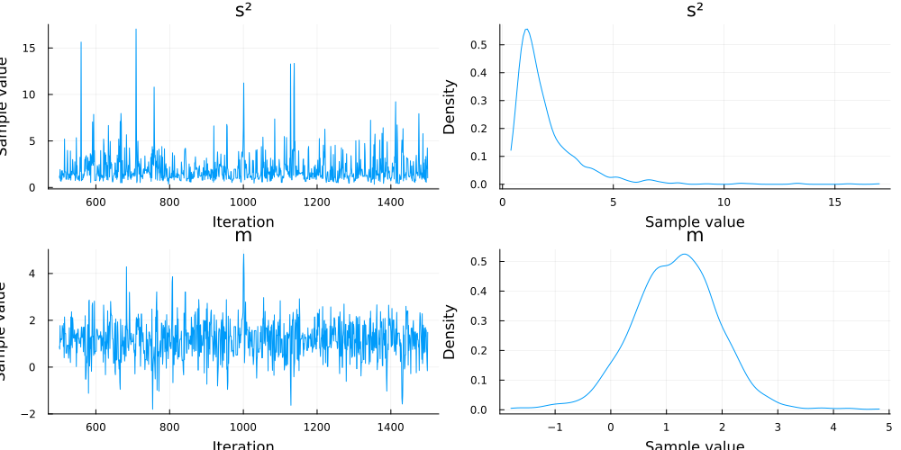
We can plot the results
plot(chn)
In this case, because we use the normal-inverse gamma distribution as a conjugate prior, we can compute its updated mean as follows:
s² = InverseGamma(2, 3)
m = Normal(0, 1)
data = [1.5, 2]
x_bar = mean(data)
N = length(data)

mean_exp = (m.σ * m.μ + N * x_bar) / (m.σ + N)
1.1666666666666667
We can also compute the updated variance
updated_alpha = shape(s²) + (N / 2)
updated_beta =
    scale(s²) +
    (1 / 2) * sum((data[n] - x_bar)^2 for n in 1:N) +
    (N * m.σ) / (N + m.σ) * ((x_bar)^2) / 2
variance_exp = updated_beta / (updated_alpha - 1)
2.0416666666666665
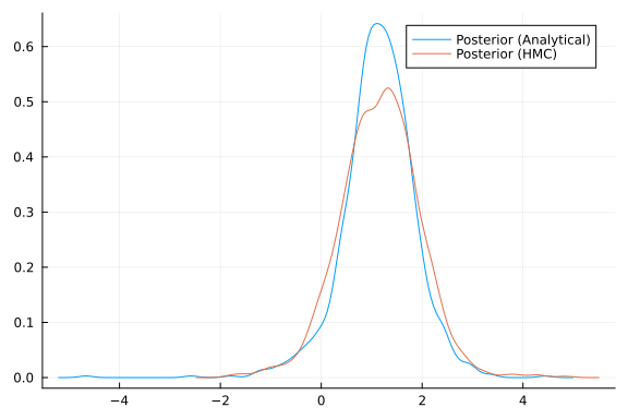
Finally, we can check if these expectations align with our HMC approximations from earlier. We can compute samples from a normal-inverse gamma following the equations given here.
function sample_posterior(alpha, beta, mean, lambda, iterations)
    samples = []
    for i in 1:iterations
        sample_variance = rand(InverseGamma(alpha, beta), 1)
        sample_x = rand(Normal(mean, sqrt(sample_variance[1]) / lambda), 1)
        sanples = append!(samples, sample_x)
    end
    return samples
end

analytical_samples = sample_posterior(updated_alpha, updated_beta, mean_exp, 2, 1000);
density(analytical_samples; label="Posterior (Analytical)")
density!(chn[:m]; label="Posterior (HMC)")