Probabilistic Programming in Thirty Seconds

If you are already well-versed in probabilistic programming and want to take a quick look at how Turing's syntax works or otherwise just want a model to start with, we have provided a complete Bayesian coin-flipping model below.

This example can be run wherever you have Julia installed (see Getting Started), but you will need to install the packages Turing and StatsPlots if you have not done so already.

This is an excerpt from a more formal example which can be found in this Jupyter notebook or as part of the documentation website here.

# Import libraries.
using Turing, StatsPlots, Random

# Set the true probability of heads in a coin.
p_true = 0.5

# Iterate from having seen 0 observations to 100 observations.
Ns = 0:100

0:100

# Draw data from a Bernoulli distribution, i.e. draw heads or tails.
Random.seed!(12)
data = rand(Bernoulli(p_true), last(Ns))

100-element Vector{Bool}:
 1
 0
 0
 0
 1
 1
 1
 0
 1
 0
 ⋮
 0
 1
 0
 0
 1
 0
 0
 0
 1

# Declare our Turing model.
@model function coinflip(y)
    # Our prior belief about the probability of heads in a coin.
    p ~ Beta(1, 1)

    # The number of observations.
    N = length(y)
    for n in 1:N
        # Heads or tails of a coin are drawn from a Bernoulli distribution.
        y[n] ~ Bernoulli(p)
    end
end

coinflip (generic function with 2 methods)

# Settings of the Hamiltonian Monte Carlo (HMC) sampler.
iterations = 1000
ϵ = 0.05
τ = 10

# Start sampling.
chain = sample(coinflip(data), HMC(ϵ, τ), iterations)

Chains MCMC chain (1000×11×1 Array{Float64, 3}):

Iterations        = 1:1:1000
Number of chains  = 1
Samples per chain = 1000
Wall duration     = 1.0 seconds
Compute duration  = 1.0 seconds
parameters        = p
internals         = lp, n_steps, is_accept, acceptance_rate, log_density, h
amiltonian_energy, hamiltonian_energy_error, numerical_error, step_size, no
m_step_size

Summary Statistics
  parameters      mean       std      mcse    ess_bulk   ess_tail      rhat
    ⋯
      Symbol   Float64   Float64   Float64     Float64    Float64   Float64
    ⋯

           p    0.4311    0.0475    0.0009   3000.0000   602.0565    1.0010
    ⋯
                                                                1 column om
itted

Quantiles
  parameters      2.5%     25.0%     50.0%     75.0%     97.5%
      Symbol   Float64   Float64   Float64   Float64   Float64

           p    0.3404    0.3977    0.4304    0.4633    0.5241

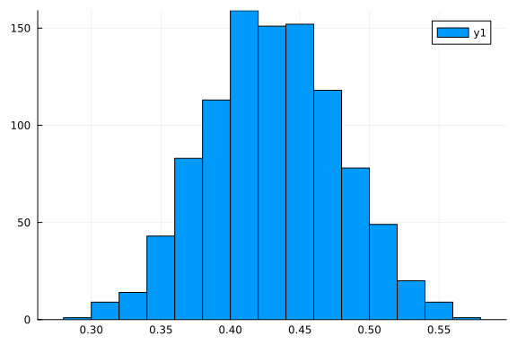
# Plot a summary of the sampling process for the parameter p, i.e. the probability of heads in a coin.
histogram(chain[:p])