Probabilistic Principal Component Analysis (p-PCA)
Overview of PCA
Principal component analysis (PCA) is a fundamental technique to analyse and visualise data. It is an unsupervised learning method mainly used for dimensionality reduction.
For example, we have a data matrix $\mathbf{X} \in \mathbb{R}^{N \times D}$, and we would like to extract $k \ll D$ principal components which captures most of the information from the original matrix. The goal is to understand $\mathbf{X}$ through a lower dimensional subspace (e.g. two-dimensional subspace for visualisation convenience) spanned by the principal components.
In order to project the original data matrix into low dimensions, we need to find the principal directions where most of the variations of $\mathbf{X}$ lie in. Traditionally, this is implemented via singular value decomposition (SVD) which provides a robust and accurate computational framework for decomposing matrix into products of rotation-scaling-rotation matrices, particularly for large datasets(see an illustration here):
$$ \mathbf{X}{N \times D} = \mathbf{U}{N \times r} \times \boldsymbol{\Sigma}{r \times r} \times \mathbf{V}^T{r \times D} $$
where $\Sigma_{r \times r}$ contains only $r := \operatorname{rank} \mathbf{X} \leq \min{N,D}$ non-zero singular values of $\mathbf{X}$. If we pad $\Sigma$ with zeros and add arbitrary orthonormal columns to $\mathbf{U}$ and $\mathbf{V}$, we obtain the more compact form:[^1]
$$ \mathbf{X}{N \times D} = \mathbf{U}{N \times N} \mathbf{\Sigma}{N \times D} \mathbf{V}{D \times D}^T $$
where $\mathbf{U}$ and $\mathbf{V}$ are unitary matrices (i.e. with orthonormal columns). Such a decomposition always exists for any matrix. Columns of $\mathbf{V}$ are the principal directions/axes. The percentage of variations explained can be calculated using the ratios of singular values.[^3]
Here we take a probabilistic perspective. For more details and a mathematical derivation, we recommend Bishop's textbook (Christopher M. Bishop, Pattern Recognition and Machine Learning, 2006). The idea of proabilistic PCA is to find a latent variable $z$ that can be used to describe the hidden structure in a dataset.[^2] Consider a data set $\mathbf{X}_{D \times N}={x_i}$ with $i=1,2,...,N$ data points, where each data point $x_i$ is $D$-dimensional (i.e. $x_i \in \mathcal{R}^D$). Note that, here we use the flipped version of the data matrix. We aim to represent the original $n$ dimensional vector using a lower dimensional a latent variable $z_i \in \mathcal{R}^k$.
We first assume that each latent variable $z_i$ is normally distributed:
$$ z_i \sim \mathcal{N}(0, I) $$
and the corresponding data point is generated via projection:
$$ x_i | z_i \sim \mathcal{N}(\mathbf{W} z_i + \boldsymbol{μ}, \sigma^2 \mathbf{I}) $$
where the projection matrix $\mathbf{W}{D \times k}$ accommodates the principal axes.
The above formula expresses $x_i$ as a linear combination of the basis columns in the projection matrix W, where the combination coefficients sit in z_i (they are the coordinats of x_i in the new $k$-dimensional space.).
We can also express the above formula in matrix form: $\mathbf{X}{D \times N} \approx \mathbf{W}{D \times k} \mathbf{Z}{k \times N}$.
We are interested in inferring $\mathbf{W}$, $μ$ and $\sigma$.
Classical PCA is the specific case of probabilistic PCA when the covariance of the noise becomes infinitesimally small, i.e. $\sigma^2 \to 0$. Probabilistic PCA generalizes classical PCA, this can be seen by marginalizing out the the latent variable.[^2]
The gene expression example
In the first example, we illustrate:
- how to specify the probabilistic model and
- how to perform inference on $\mathbf{W}$, $\boldsymbol{\mu}$ and $\sigma$ using MCMC.
We use simulated gemnome data to demonstrate these. The simulation is inspired by biological measurement of expression of genes in cells, and each cell is characterized by different gene features. While the human genome is (mostly) identical between all the cells in the body, there exist interesting differences in gene expression in different human tissues and disease conditions. One way to investigate certain diseases is to look at differences in gene expression in cells from patients and healthy controls (usually from the same tissue).
Usually, we can assume that the changes in gene expression only affect a subset of all genes (and these can be linked to diseases in some way). One of the challenges for this kind of data is to explore the underlying structure, e.g. to make the connection between a certain state (healthy/disease) and gene expression. This becomes difficult when the dimensions is very large (up to 20000 genes across 1000s of cells). So in order to find structure in this data, it is useful to project the data into a lower dimensional space.
Regardless of the biological background, the more abstract problem formulation is to project the data living in high-dimensional space onto a representation in lower-dimensional space where most of the variation is concentrated in the first few dimensions. We use PCA to explore underlying structure or pattern which may not necessarily be obvious from looking at the raw data itself.
Step 1: configuration of dependencies
First, we load the dependencies used.
using Turing
using ReverseDiff
Turing.setadbackend(:reversediff)
using LinearAlgebra, FillArrays

# Packages for visualization
using DataFrames, StatsPlots, Measures

# Set a seed for reproducibility.
using Random
Random.seed!(1789);
All packages used in this tutorial are listed here.
You can install them via using Pkg; Pkg.add("package_name").
Package usages:
We use
DataFramesfor instantiating matrices,LinearAlgebraandFillArraysto perform matrix operations;Turingfor model specification and MCMC sampling,ReverseDifffor setting the automatic differentiation backend when sampling.StatsPlotsfor visualising the resutls., Measuresfor setting plot margin units. As all examples involve sampling, for reproducibility we set a fixed seed using theRandomstandard library.
Step 2: Data generation
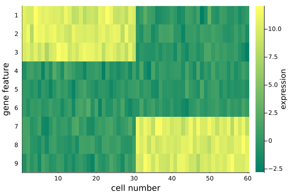
Here, we simulate the biological gene expression problem described earlier. We simulate 60 cells, each cell has 9 gene features. This is a simplified problem with only a few cells and genes for demonstration purpose, which is not comparable to the complexity in real-life (e.g. thousands of features for each individual). Even so, spotting the structures or patterns in a 9-feature space would be a challenging task; it would be nice to reduce the dimentionality using p-PCA.
By design, we mannually divide the 60 cells into two groups. the first 3 gene features of the first 30 cells have mean 10, while those of the last 30 cells have mean 10. These two groups of cells differ in the expression of genes.
n_genes = 9 # D
n_cells = 60 # N

# create a diagonal block like expression matrix, with some non-informative genes;
# not all features/genes are informative, some might just not differ very much between cells)
mat_exp = randn(n_genes, n_cells)
mat_exp[1:(n_genes ÷ 3), 1:(n_cells ÷ 2)] .+= 10
mat_exp[(2 * (n_genes ÷ 3) + 1):end, (n_cells ÷ 2 + 1):end] .+= 10
3×30 view(::Matrix{Float64}, 7:9, 31:60) with eltype Float64:
 11.3047   9.46905  11.112   10.254    …   9.39734  11.0083    8.30576
 11.1976   9.979    10.7737   8.56915     10.3514   12.0768   10.3927
  9.99143  9.40082  11.8372  10.9009       9.88801   9.75763  10.6981
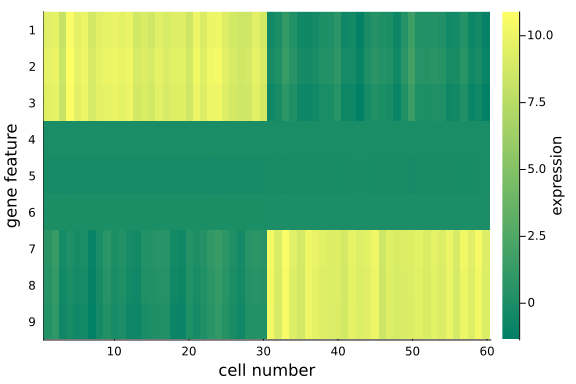
To visualize the $(D=9) \times (N=60)$ data matrix mat_exp, we use the heatmap plot.
heatmap(
    mat_exp;
    c=:summer,
    colors=:value,
    xlabel="cell number",
    yflip=true,
    ylabel="gene feature",
    yticks=1:9,
    colorbar_title="expression",
)
Note that:
- We have made distinct feature differences between these two groups of cells (it is fairly obvious from looking at the raw data), in practice and with large enough data sets, it is often impossible to spot the differences from the raw data alone.
- If you have some patience and compute resources you can increase the size of the dataset, or play around with the noise levels to make the problem increasingly harder.
Step 3: Create the pPCA model
Here we construct the probabilistic model pPCA().
As per the p-PCA formula, we think of each row (i.e. each gene feature) following a $N=60$ dimensional multivariate normal distribution centered around the corresponding row of $\mathbf{W}{D \times k} \times \mathbf{Z}{k \times N} + \boldsymbol{\mu}_{D \times N}$.
@model function pPCA(X::AbstractMatrix{<:Real}, k::Int)
    # retrieve the dimension of input matrix X.
    N, D = size(X)

    # weights/loadings W
    W ~ filldist(Normal(), D, k)

    # latent variable z
    Z ~ filldist(Normal(), k, N)

    # mean offset
    μ ~ MvNormal(Eye(D))
    genes_mean = W * Z .+ reshape(μ, n_genes, 1)
    return X ~ arraydist([MvNormal(m, Eye(N)) for m in eachcol(genes_mean')])
end;
The function pPCA() accepts:
- an data array $\mathbf{X}$ (with no. of instances x dimension no. of features, NB: it is a transpose of the original data matrix);
- an integer $k$ which indicates the dimension of the latent space (the space the original feature matrix is projected onto).
Specifically:
- it first extracts the dimension $D$ and number of instances $N$ of the input matrix;
- draw samples of each entries of the projection matrix $\mathbf{W}$ from a standard normal;
- draw samples of the latent variable $\mathbf{Z}_{k \times N}$ from an MND;
- draw samples of the offset $\boldsymbol{\mu}$ from an MND, assuming uniform offset for all instances;
- Finally, we iterate through each gene dimension in $\mathbf{X}$, and define an MND for the sampling distribution (i.e. likelihood).
Step 4: Sampling-based inference of the pPCA model
Here we aim to perform MCMC sampling to infer the projection matrix $\mathbf{W}{D \times k}$, the latent variable matrix $\mathbf{Z}{k \times N}$, and the offsets $\boldsymbol{\mu}_{N \times 1}$.
We run the inference using the NUTS sampler, of which the chain length is set to be 500, target accept ratio 0.65 and initial stepsize 0.1. By default, the NUTS sampler samples 1 chain. You are free to try different samplers.
k = 2 # k is the dimension of the projected space, i.e. the number of principal components/axes of choice
ppca = pPCA(mat_exp', k) # instantiate the probabilistic model
chain_ppca = sample(ppca, NUTS(), 500);
The samples are saved in the Chains struct chain_ppca, whose shape can be checked:
size(chain_ppca) # (no. of iterations, no. of vars, no. of chains) = (500, 159, 1)
(500, 159, 1)
The Chains struct chain_ppca also contains the sampling info such as r-hat, ess, mean estimates, etc.
You can print it to check these quantities.
Step 5: posterior predictive checks
We try to reconstruct the input data using the posterior mean as parameter estimates.
We first retrieve the samples for the projection matrix W from chain_ppca. This can be done using the Julia group(chain, parameter_name) function.
Then we calculate the mean value for each element in $W$, averaging over the whole chain of samples.
# Extract parameter estimates for predicting x - mean of posterior
W = reshape(mean(group(chain_ppca, :W))[:, 2], (n_genes, k))
Z = reshape(mean(group(chain_ppca, :Z))[:, 2], (k, n_cells))
μ = mean(group(chain_ppca, :μ))[:, 2]

mat_rec = W * Z .+ repeat(μ; inner=(1, n_cells))
9×60 Matrix{Float64}:
  7.26663     7.08729     7.60895     …   2.08168     1.81392     2.12189
  7.49552     7.31816     7.8329          2.36028     2.09297     2.39907
  7.26867     7.0855      7.61725         1.96631     1.69058     2.0065
 -0.018629   -0.0226136  -0.00946715     -0.123628   -0.126209   -0.121423
 -0.31514    -0.311867   -0.321854       -0.223586   -0.219711   -0.224714
  0.0403905   0.0376105   0.0461812   …  -0.0368092  -0.0399118  -0.0357777
  2.50081     2.68252     2.15469         7.75869     8.03151     7.71855
  2.47757     2.65606     2.13782         7.64405     7.91257     7.60482
  2.28059     2.46434     1.92999         7.59378     7.8684      7.55269
heatmap(
    mat_rec;
    c=:summer,
    colors=:value,
    xlabel="cell number",
    yflip=true,
    ylabel="gene feature",
    yticks=1:9,
    colorbar_title="expression",
)
We can quantitatively check the absolute magnitudes of the column average of the gap between mat_exp and mat_rec:
We observe that, using posterior mean, the recovered data matrix mat_rec has values align with the original data matrix - particularly the same pattern in the first and last 3 gene features are captured, which implies the inference and p-PCA decomposition are successful.
This is satisfying as we have just projected the original 9-dimensional space onto a 2-dimensional space - some info has been cut off in the projection process, but we haven't lost any important info, e.g. the key differences between the two groups.
The is the desirable property of PCA: it picks up the principal axes along which most of the (original) data variations cluster, and remove those less relevant.
If we choose the reduced space dimension $k$ to be exactly $D$ (the original data dimension), we would recover exactly the same original data matrix mat_exp, i.e. all information will be preserved.
Now we have represented the original high-dimensional data in two dimensions, without lossing the key information about the two groups of cells in the input data.
Finally, the benefits of performing PCA is to analyse and visualise the dimension-reduced data in the projected, low-dimensional space.
we save the dimension-reduced matrix $\mathbf{Z}$ as a DataFrame, rename the columns and visualise the first two dimensions.
df_pca = DataFrame(Z', :auto)
rename!(df_pca, Symbol.(["z" * string(i) for i in collect(1:k)]))
df_pca[!, :type] = repeat([1, 2]; inner=n_cells ÷ 2)
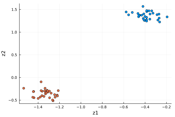
scatter(df_pca[:, :z1], df_pca[:, :z2]; xlabel="z1", ylabel="z2", group=df_pca[:, :type])
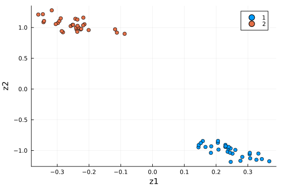
We see the two groups are well separated in this 2-D space. As an unsupervised learning method, performing PCA on this dataset gives membership for each cell instance. Another way to put it: 2 dimensions is enough to capture the main structure of the data.
Further extension: automatic choice of the number of principal components with ARD
A direct question arises from above practice is: how many principal components do we want to keep, in order to sufficiently represent the latent structure in the data? This is a very central question for all latent factor models, i.e. how many dimensions are needed to represent that data in the latent space. In the case of PCA, there exist a lot of heuristics to make that choice. For example, We can tune the number of principal components using empirical methods such as cross-validation based some criteria such as MSE between the posterior predicted (e.g. mean predictions) data matrix and the original data matrix or the percentage of variation explained [3].
For p-PCA, this can be done in an elegant and principled way, using a technique called Automatic Relevance Determination (ARD). ARD can help pick the correct number of principal directions by regularizing the solution space using a parameterized, data-dependent prior distribution that effectively prunes away redundant or superfluous features [4]. Essentially, we are using a specific prior over the factor loadings $\mathbf{W}$ that allows us to prune away dimensions in the latent space. The prior is determined by a precision hyperparameter $\alpha$. Here, smaller values of $\alpha$ correspond to more important components. You can find more details about this in e.g. [5].
@model function pPCA_ARD(X)
    # Dimensionality of the problem.
    N, D = size(X)

    # latent variable Z
    Z ~ filldist(Normal(), D, N)

    # weights/loadings w with Automatic Relevance Determination part
    α ~ filldist(Gamma(1.0, 1.0), D)
    W ~ filldist(MvNormal(zeros(D), 1.0 ./ sqrt.(α)), D)

    mu = (W' * Z)'

    tau ~ Gamma(1.0, 1.0)
    return X ~ arraydist([MvNormal(m, 1.0 / sqrt(tau)) for m in eachcol(mu)])
end;
Instead of drawing samples of each entry in $\mathbf{W}$ from a standard normal, this time we repeatedly draw $D$ samples from the $D$-dimensional MND, forming a $D \times D$ matrix $\mathbf{W}$. This matrix is a function of $\alpha$ as the samples are drawn from the MND parameterized by $\alpha$. We also introduce a hyper-parameter $\tau$ which is the precision in the sampling distribution. We also re-paramterise the sampling distribution, i.e. each dimension across all instances is a 60-dimensional multivariate normal distribution. Re-parameterisation can sometimes accelrate the sampling process.
We instantiate the model and ask Turing to sample from it using NUTS sampler. The sample trajectories of $\alpha$ is plotted using the plot function from the package StatsPlots.
ppca_ARD = pPCA_ARD(mat_exp') # instantiate the probabilistic model
chain_ppcaARD = sample(ppca_ARD, NUTS(), 500) # sampling
plot(group(chain_ppcaARD, :α); margin=6.0mm)
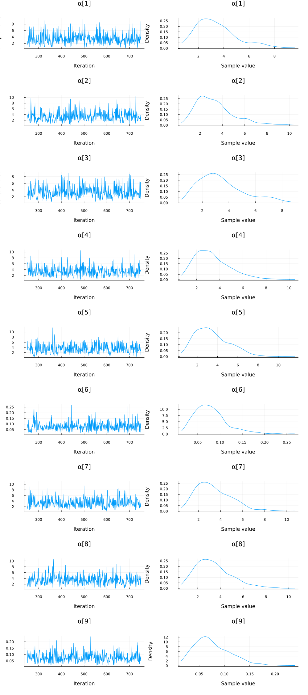
Again, we do some inference diagnostics. Here we look at the convergence of the chains for the $α$ parameter. This parameter determines the relevance of individual components. We see that the chains have converged and the posterior of the $\alpha$ parameters is centered around much smaller values in two instances. In the following, we will use the mean of the small values to select the relevant dimensions (remember that, smaller values of $\alpha$ correspond to more important components.). We can clearly see from the values of $\alpha$ that there should be two dimensions (corresponding to $\bar{\alpha}_3=\bar{\alpha}_5≈0.05$) for this dataset.
# Extract parameter mean estimates of the posterior
W = permutedims(reshape(mean(group(chain_ppcaARD, :W))[:, 2], (n_genes, n_genes)))
Z = permutedims(reshape(mean(group(chain_ppcaARD, :Z))[:, 2], (n_genes, n_cells)))'
α = mean(group(chain_ppcaARD, :α))[:, 2]
plot(α; label="α")
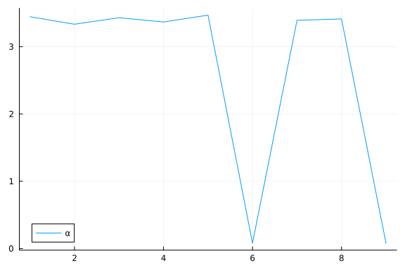
We can inspect α to see which elements are small (i.e. high relevance).
To do this, we first sort α using sortperm() (in ascending order by default), and record the indices of the first two smallest values (among the $D=9$ $\alpha$ values).
After picking the desired principal directions, we extract the corresponding subset loading vectors from $\mathbf{W}$, and the corresponding dimensions of $\mathbf{Z}$.
We obtain a posterior predicted matrix $\mathbf{X} \in \mathbb{R}^{2 \times 60}$ as the product of the two sub-matrices, and compare the recovered info with the original matrix.
α_indices = sortperm(α)[1:2]
k = size(α_indices)[1]
X_rec = W[:, α_indices] * Z[α_indices, :]
df_rec = DataFrame(X_rec', :auto)
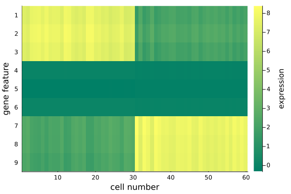
heatmap(
X_rec;
c=:summer,
colors=:value,
xlabel="cell number",
yflip=true,
ylabel="gene feature",
yticks=1:9,
colorbar_title="expression",
)
We observe that, the data in the original space is recovered with key information, the distinct feature values in the first and last three genes for the two cell groups, are preserved. We can also examine the data in the dimension-reduced space, i.e. the selected components (rows) in $\mathbf{Z}$.
df_pro = DataFrame(Z[α_indices, :]', :auto)
rename!(df_pro, Symbol.(["z" * string(i) for i in collect(1:k)]))
df_pro[!, :type] = repeat([1, 2]; inner=n_cells ÷ 2)
scatter(
    df_pro[:, 1], df_pro[:, 2]; xlabel="z1", ylabel="z2", color=df_pro[:, "type"], label=""
)
This plot is very similar to the low-dimensional plot above, with the relevant dimensions chosen based on the values of $α$ via ARD. When you are in doubt about the number of dimensions to project onto, ARD might provide an answer to that question.
Final comments.
p-PCA is a linear map which linearly transforms the data between the original and projected spaces. It can also thought as a matrix factorisation method, in which $\mathbf{X}=(\mathbf{W} \times \mathbf{Z})^T$. The projection matrix can be understood as a new basis in the projected space, and $\mathbf{Z}$ are the new coordinates.
References:
[^1]: Gilbert Strang, Introduction to Linear Algebra, 5th Ed., Wellesley-Cambridge Press, 2016. [^2]: Probabilistic PCA by TensorFlow, "https://www.tensorflow.org/probability/examples/Probabilistic_PCA". [^3]: Gareth M. James, Daniela Witten, Trevor Hastie, Robert Tibshirani, An Introduction to Statistical Learning, Springer, 2013. [^4]: David Wipf, Srikantan Nagarajan, A New View of Automatic Relevance Determination, NIPS 2007. [^5]: Christopher Bishop, Pattern Recognition and Machine Learning, Springer, 2006.